Welcome to DNA land. Most of us here have been curious about DNA testing and how it can help discover relatives. We chose a testing service and sent in a sample of our DNA. The testing service sent us back a list of predicted relatives who also tested with their service. They also allow us to download our ‘raw file’, a characterization of some parts our actual DNA. Now what?
Somewhere in that information are connections to cousins we have never met, and the secrets of our ancestors’ identities; e.g. a 3rd g-grandmother may be lurking there in DNA form, waiting to be reconnected with her descendants. This article discusses how to do that, by exploring how DNA matching can help us identify a common ancestor (CA) with someone who shares parts of our DNA. The descendants of that common ancestor are either our cousins or ancestors.
This article is technical. Review concepts, terminology, and acronyms here.
Analyzing DNA results – GEDmatch and Support Resources
Currently, the largest fee-based DNA testing companies are 23&Me, MyHeritage, FTDNA, and Ancestry. I chose 23andMe purely based on their marketing style. Other companies do all types of gaming of their customer base to increase revenue streams; every slice of information has its little price. 23andMe keeps it simple; charge a fair price for the test, and support free interchange of information. Companies that are respectful of their customers get my business.
Such companies will sample our DNA, then provide a raw data file of our maximal likelihood DNA results (increasingly imputed!). This testing identifies only a brief sampling of a few hundred thousand alleles (markers), and so does not offer the same order accuracy as a full genome test, or even an exome test. And as imputation algorithms become more refined and powerful, testing companies are testing fewer markers, for ancestry determination, than they did five years ago.
The raw data file is interpreted by online tools provided by the testing company, allowing one to compare with others at that testing service. Most customers will have no direct interface to their raw data file, except to share their genome data with a different analysis provider, usually the GEDmatch service, although the companies are now each accepting the others’ DNA file uploads as well (23andMe does not).
Even within a testing company, the methodology changes rapidly, so customers who test at different times will have different markers tested. Imputation will be needed to fill in all the blanks in order to compare customers who tested with different variants of the technology.
Just as intra-company testing varies as technology changes, inter-company testing results in further difference in data collection. One cannot reliably find relatives by matching results from different testing regimes unless sufficient analysis and imputation is performed first, to ensure comparisons are between equivalent data. See this ISOGG Chart for counts of the tested parameters of each major testing firm, and the degree to which each test overlaps with the competitors’ tests.
GEDmatch is a mostly free analysis service (advanced tools available for small fee) that does no testing itself, but allows cross-comparing results from the different testing services. Simply download your raw results from your testing service and upload them to GEDmatch. Many people have migrated their results to GEDmatch, so it is the place to go to get the biggest bang for one’s DNA comparisons. But there is added risk of inaccuracy as well, since the raw data being compared is not entirely compatible, adding another layer of imputation.
The terms imputed and maximal likelihood should raise a red flag with us that tested DNA results for genealogical use are increasingly statistical in nature. The testing companies’ main customers are involved in disease research, where a guess at an allele, based on other DNA knowledge, likely would not be solid grounds to predict a serious disease susceptibility. So technology is veering noticeably toward providing hard evidence for disease prediction, discovery and treatment; genealogy, the lesser DNA client, must increasingly impute values of interest from the hard evidence of the favored DNA client.
Imputation works reasonably well with DNA, because DNA is not random. It is a blueprint for a finely tuned machine, and the various parts are interconnected in ways beyond the reach of our current analysis. The term linkage disequilibrium (LD) refers to the non-random couplings evidenced between otherwise independent alleles; the entire mechanism is not yet within our focus.
GEDmatch also provides a facility for accepting and displaying paper genealogy trees, via the GEDCOM standard or via direct link to Wikitree, the free global genealogy tree site. Using DNA to locate specific CAs cannot work if relatives don’t have the associated paper trails to identify the matches. DNA contains no names and places. We need to have done the leg work.
Many 23andMe customers have uploaded their DNA to GEDmatch, so most matching can be done at GEDmatch; only residual matching will be required at 23andMe directly. GEDmatch provides Tier 1 (paid) tools to assist in grouping DNA relatives based on shared common ancestors, the process called triangulation. There are likely other tools available also. But a spreadsheet and the standard (free) tools of 23andMe and GEDmatch suffice for my purposes.
DNA analysis tools will be difficult to utilize, or even comprehend, without some knowledge of the lay of DNA land. We have to get our hands a little dirty to make our DNA reveal what it knows about us, which is a lot.
Genetic Background – How We Inherit Our DNA
Autosomal DNA (atDNA or auDNA) is another term for recombinant DNA, the DNA that is inherited as 22 pairs of recombining chromosomes (autosomes). Each pair consists of one chromosome from each parent. Each of these two chromosomes contains a mix of DNA (genes) from the respective grandparents. We call a heritable section of DNA a segment.
This mixing of DNA segments is called crossover. It occurs in an early phase of the complex, multi-stage meiosis process, during gamete (human germ cell, sperm or egg) production. The details are not germane here; see ‘Fat Alberts’, or other online discussions. Below, our use of ‘chromosome’ refers specifically to autosomal chromosomes numbered 1-22.
How can one chromosome from a single parent represent both respective grandparents? Two or three DNA segments are usually pseudo-randomly mixed on each chromosome during meiosis crossover. There are hotspots and coldspots on each chromosome where such splicing is more often or less often performed. When a gamete joins an oppositely-sexed gamete during fertilization, the resulting offspring’s atDNA consists of paired chromosomes, each consisting of mixed segments representing the parents of its donor, the offspring’s maternal and paternal grandparents.
Combined with the 223 different configurations of human gamete that can be expressed during meiosis (a father or mother choice for each chromosome), it is clear that meiosis is a source of great DNA shuffling, and explains why non-twinned children of the same parents are so unique.
Meiosis guarantees that no ancestor gets left out of one’s DNA in near-by generations, but by the 6th generation back, the theoretical probability of having all 64 ancestors represented in one’s DNA becomes vanishingly small:
- 100% chance of representing all 4 grandparents
- 96% chance of representing all 16 g-g-grandparents
- 54% chance of representing all 32 g-g-g-grandparents
- .01% chance of representing all 64 g-g-g-g-grandparents
Another way of looking at this is through percent of DNA passed down. For example, the descendants of an ancestor living 12 generations ago will share less and less of her total ancestry going forward:
- gen 3: 97%
- gen 5: 74%
- gen 7: 45%
- gen 9: 19%
- gen 11: 6%
The above percentages vary according to size and other characteristics of an ancestral population. Here they are averages over three separate pedigree populations.
Inheritance of Crossover Segments Over The Generations
Summarizing the above, a chromosome in a human gamete is inherited from the source parent who produced it. During meiosis, at least one, and often two segments of DNA on a gamete chromosome are sourced from the chromosome provided by the other parent. Thus, both sets of grandparents are represented in each inherited chromosome pair. Following is a simplified graphic of the division of the inherited genome over the generations; the top line are the g-g-grandparents of the siblings at the bottom (unattributed file scraped from the Internet):
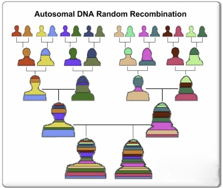
Each crossover event divides some of a chromosome’s segments into shorter heritable segments. All segments of the same color are identical segments of the original g-g-grandparent DNA of that color. Thus, the length of a segment attributable to a specific ancestor is related to the number of ancestral generations that have intervened since that ancestor.
Note: To be statistically accurate, the siblings (bottom row) should have only 15 color stripes. Already, some grandparent contributions are likely to have disappeared from their g-g-grandchildrens’ genomes.
What do we mean by segment length? There are different measures of chromosomal length:
- number of base pairs (BP)
- number of single nucleotide polymorphisms (SNP)
- number of centiMorgans (cM).
A cM is not actually a fixed measure of DNA BPs, but rather a probabilistic measure that accommodates the hot and cold spots mentioned previously. 1 cM is defined as the amount of location-specific DNA for which there exists a 1% probability of its containing a segment crossover point. The average chromosome length is ~160 cM. Since there is, by definition and the ‘rules’ of meiosis, a 100% probability that a crossover point will occur in 100cM, all chromosomes are ensured to host one crossover segment; thus one can say no grandparent will be left behind.
The resulting alternating-parent DNA segments on a chromosome each consists of many millions of BPs, several thousands of SNPs, and measures many tens of centiMorgans (cM) in length, a count that varies widely in differing chromosome regions, and surprisingly, even between M/F gametes.
How Are Common Ancestors Identified By Inherited DNA Segments?
If two persons share an entire chromosome after crossover, it is likely they will be siblings; the parent will be the CA. If a significant part of a chromosome is shared, it is likely the sharing pair will be first cousins, with a grandparent as the CA. The further removed in ancestry one is from the genome being matched, the smaller the segment that will be shared.
It is nirvana to find an ancestor by segment matching. Yet not all segment matches are productive. There are two qualities of match when comparing shared chromosome segments, Identity by Descent (IBD), and Identity by State (IBS). All ancestor identification is via IBD matching, where the matching genomes have at least one near-term CA. However, it is possible to match a segment, but for the two parties not to share a recent CA. This is IBS, and can occur when a segment descends from multiple sources having different ancestry, but by chance matches the comparison genome (aka IBC, inheritance by chance).
When an IBD shared segment is found in common between two relatives, the end points of each relative’s chromosome segment will likely be different. What is actually shared is the overlap between the two chromosome segments. Further, this overlap area may itself be shared by other relatives with the same or different CA. The term ‘segmentology’ has been devised to describe the determination of common ancestors from shared DNA segments.
In segmentology used for determining a CA, one is usually looking at segment lengths between 25 and 125 cM, or 0.4% to 2% of shared DNA. Shared segments larger than that will likely have readily apparent ancestral sources. Smaller segments refer to more distant ancestors for which a paper tree is unlikely to be available linking the ancestor to the current generation. The statistical ancestral relations corresponding to these lengths are:
- 1.6% shared DNA or 110 cM – second cousins once removed, half second cousins, first cousin three times removed, half first cousin twice removed
- 0.8% shared DNA or 55 cM – third cousins, second cousins twice removed
- 0.4% shared DNA or 27 cM – third cousins once removed
These are statistical because for shorter shared segments, there is greater chance they will lie in a section of the chromosome where entire short segments are inherited in an all-or-nothing manner. Therefore, a third, fourth, fifth, or sixth cousin could inherit the same segment. This may explain why testing companies give a wider range of likely CA generation, as in third to sixth cousin, based on one short shared segment.
Heuristically, for matching segments larger than ~10cM (usually indicating a 4th-5th cousin or closer relationship), there is scant evidence of false positives through IBS. It is generally safe to assume IBD and to pursue identification of the CA. But evidence suggests that a segment match of ~7cM length has a 50-50 chance of being an IBS match. For such shorter segments, typically shared by > 5C-distant relations, extra information may be needed to determine if there is a recent CA, via the triangulation process described below, used to weed out false positives.
In my own nascent research, 3C2R is the furthest relative I have matched for which a paper trail connected us, allowing me to prove we share g-g-grandparents as our CA. Thus were my father’s father’s father’s father and mother proven as my biological ancestors.
Here, I had no common segments with this match, but my sibling shared a somewhat large 65cM segment of one chromosome with her, divided into two nearly adjacent segments. This combined segment length is more than twice what the table above predicts for 3C2R relationships (although it did consist of two smaller distinct segments that were close by each other).
Methodology
Triangulation matching is used to weed out IBS false positives that wrongly suggest a recent CA. Triangulation can further define which relatives belong to which CA, a process called triangulation grouping. Triangulation requires, as a first step, finding all one’s registered-DNA relatives via search for shared DNA segments on all 22 autosome pairs. The second step is to compare all persons who match you with one another. Some will not match some others, even though they all match you, because we each inherit a chromosome from each parent; one person’s match on father’s chromosome, and another person’s match on mother’s chromosome, will both match you, but may not be related to each another.
From the main page after logging into GEDmatch, request the One-to-many report (free) from the Data Analysis panel, with segment length threshold set to 10 cM (default is 7 cM). This produces a table of people matching your DNA at some level. Copy the data columns of this report to your spreadsheet.
The table has a select column, and one must check it for each row entry for which detailed chromosome comparisons are wanted, which should be all people above a certain threshold of total segment length of matching DNA. I chose all people with total segment matching length of >23cM. That was over 150 people, a tedious selection process. Save this page with selections made, so you don’t have to redo the selections if you want to re-run the analysis. The Gedmatch paid triangulation tool seems to relate all persons having total shared segments length >15.5 cM, but I didn’t need that much resolution in my initial manual attempt at triangulation.
When all selections boxes are checked, click the Submit button near the top of the report page. The next page offers a choice of 2-D or 3-D chromosome browser. Select 2-D, then on the next page click on the word HERE. The result is a report of all shared segments in chromosome order, with graphic representation as well.
Go through this report and enter the segment detailed data (segment start position, end position, and length) into new columns in the spreadsheet. For easier readability, convert all segment locations to mbp units by dividing the displayed locations in base pairs by 1 million. Some on the list are duplicates or siblings with the same DNA. Remove these for a cleaner result.
A person with multiple matching chromosome segments will need a separate row for each matching segment; repeat rows as required to hold the data for each new shared segment. Remove any rows corresponding to individual segments less than 10 cM in length. (I allowed segments >8.5 cM if the same person had an adjacent segment >10cM, gaining a few more data points). Most segments smaller than 7 cM seem to be IBS matches, and they will confuse the process going forward; it is recommended they be culled.
Return to 23andMe (or whatever other DNA sites were used) to pick up the data for those relatives who had not uploaded their DNA to GEDmatch. On 23andMe, I matched their DNA individually with mine using the DNA tab, then copied the detailed matching segment data to the spreadsheet.
The spreadsheet has now expanded, with a row for each segment shared with me, for each person matching my DNA who had registered in GEDmatch and 23&Me. I ended up with 115 distinct relatives sharing with me over 150 DNA distinct segments > 8.5 cM, spread over all 22 autosomes.
The next step is to consolidate (roll-up) and name the prospective shared segments, eliminating duplication and thus simplifying the process going forward. Consolidation consists of rolling up overlapping, nested segments on a chromosome and noting the greatest start location and least end location for each distinct set of nested segments. Some judgement will be required regarding whether adjacent areas should be included, or excluded into their own distinct shared segment.
I chose a numeric name format xxyyyzzz for my rolled-up segments, where xx is the chromosome#, yyy and zzz are the segment start and end locations (mbp). This numeric format allows sorting rows by segment names, enabling our end game – organizing the table into mutually exclusive family groups, each rolled-up segment corresponding to a prospective common ancestor (CA), a set of g-, g-g- or g-g-g-grandparents whose segments are inherited. I ended up with approximately 50 unified (rolled-up) segment names, call them triangulated segments (TG).
Finally, one needs to consolidate TGs into a set of CA groups, each group associated with the same set of common ancestors. Find all relatives that share a TG and check which other TGs they share with anyone else. Then bring all people who share any of those TGs into the CA group and repeat, until there are no more connections to follow. My ~50 TGs comprise 11 identified, mutually-exclusive CA groupings, with about 25 uncategorized TGs left over. Each CA grouping is independent of the others (i.e. comparing people in different CA groupings revealed no IBD ancestry links).
Now that all DNA relatives identified within 5 generations or so are sorted into mutually exclusive ancestry groups associated with specific ancestral lineages, we complete the process of triangulation by comparing the people in each group with one another. While doing these binary comparisons, additional segments are added as rows to the spreadsheet, identified by the two names that share them.
My spreadsheet, after sorting and colorizing by CA groupings, appears as follows:


where the column headers are:
Kit#, Sex, TG, Start, End, cM, Name (encoded for privacy)
TG, Start, End, and Length (cM), are derived columns added to the original columns of the GEDmatch One-to-many report. A given named segment will span all the start/end segment boundaries nested within it.
In my case, I had determined three CAs by direct DNA match prior to the above sorting process. Two are common to the first large buff-colored CA group from my paternal grandfather’s lineage, one with my grandparents as CA, the other with my g-g-grandparents in the same lineage as CA. The remaining relative became associated with the sixth crimson-colored CA group, with g-grandparents as the CA from my maternal grandfather’s side. I met another match on GEDmatch, through their GEDcom match service, who shares a segment in the 8th blue-gray CA group, which is also on my maternal grandfather’s lineage, but likely seven generations back to a CA. Now I know with reasonable certainty that all the other people listed in those shared groups are associated with these same or related CAs.
23andme recently added an Ancestry Composition feature, showing one’s descent from genetically-discernible population groups (PGs). They cleverly create a pseudo-chromosome set for each such PG that reflects a typical PG genetic signature (imputation of the highest order/least specificity). By selecting a displayed PG, a color-keyed chromosome map appears, showing which of one’s chromosome segments match this pseudo-chromosome set. Below is my genetic comparison to the English-Irish PG composite genome:

One can see full and half matches just as with chromosome comparison with a specific individual. My chromosomes match just two PGs in near-term inheritance:
- English/Irish PG (Isles Descent)
- Chromosomes 2, 4, and X are full-match compares to this ancestry, while 7, 10, 16, 17, 19 are half-match compares. 23andme estimates my most recent CA within this PG are likely grandparents born between 1870 and 1910
- French/German PG (Continental Descent)
- Chromosomes 1 and 14 show full-match compares to this ancestry, while 9, 12, 18, 20 each show half-match compares. 23andme estimates my most recent CA within this PG are 2nd g-grandparents, born between 1790 and 1850.
In fact, this DNA portrait closely matches my family tree. My two most recent generations with direct linkage to Europe are my maternal grandparents from England, and my paternal 3rd g-grandfather, who came to America in 1775 from Waldeck, Hessen, Germany. The latter does not quite match 23andme’s story line, but I also have a paternal g-g-grandfather, born in NJ in 1792, (surname Bower, ancestor traced to Bayern); my father recalled a non-English language spoken in his early household life; his grandmother Bower lived with him until he was 7.
Because I know my family tree back to this set of CAs, I can tell which PG was maternal and which paternal. For my case, this feature provides a kind of poor man’s genome phasing, a means of making rough estimates when you have no access to either parent’s DNA. It may not work for everyone, but the depth of my known tree and the separate PGs defining recent paternal and maternal branches seems to create a happy phasing synergy.
I will only be able to determine its true efficacy, however, if I can identify CAs for each CA grouping and determine whether their maternal or paternal relatedness is the one predicted. So far, it’s 3/3, which is why the idea presented itself. But wouldn’t it be nice to have a more predictable methodology.
3-Sibling Phasing
For the eight CA groups whose CAs are not yet identified, but for whom I now have a predictor of which of my parents is their descendant, one could use a brute force approach to contact each person, tell them what I know, point them to my extensive tree with most all ancestors identified back to g-g-g-grandparents, and see if any of these relatives have a paper tree sufficient in depth to identify our common ancestor. This method hasn’t accomplished much to date, though.
But if three siblings have been DNA-tested, it is possible to semi-analytically determine which DNA segments match each grandparent, greatly narrowing the search area for cousins sharing segments. Some cousin searching will still be necessary to narrow the possibilities to a single grandparent. Then we will know which tree to shake to find our CA. Read more.
Related Glossary
A cell with non-paired chromosomes, such as a gamete, is called haploid. Cells with paired chromosomes are called diploid. Each chromosome pair are homologs (from homologous), identical in structure but different in content.
In addition to the 22 pairs of autosomes in each human cell, there is a 23rd pair of chromosomes called allosomes, aka the X and Y sex chromosomes. Y-chromosomes (Y-DNA) largely do not recombine during meiosis. Also, the cell mitochondria contains non-recombinant DNA, mtDNA.
An entire branch of genetic genealogy deals with such non-recombinant segments of our genomes, our Y-DNA and mt-DNA, where Y is the formal name of the male allosome, and ‘mt’ stands for mitochondria, which contains non-recombinant DNA present in all cell cytoplasm, and passed from a female to all her children via her ova.
